Three Methods of Vehicle Lateral Control: Pure Pursuit, Stanley and MPC

Explain three basic lateral control methods from theory to code and show videos in simulator

Nov 16, 2021 by Yan Ding

1. Introduction

In this article, we will discuss three methods of vehicle lateral control: Pure pursuit, Stanley, and MPC. I will also go through codes to achieve a self-driving car following a race track using these three methods respectively. The source of this project is the final assignment of the course "Introduction to self-driving cars" on Coursera[1].

2. Pure Pursuit Controller

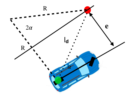
Pure pursuit is the geometric path tracking controller. A geometric path tracking controller is any controller that tracks a reference path using only the geometry of the vehicle kinematics and the reference path. Pure Pursuit controller uses a look-ahead point which is a fixed distance on the reference path ahead of the vehicle as follows. The vehicle needs to proceed to that point using a steering angle which we need to compute.

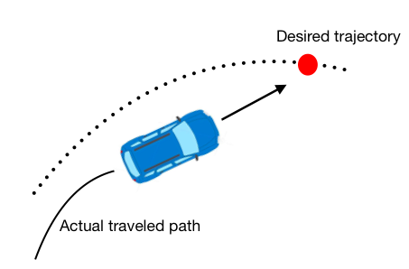
In this method, the center of the rear axle is used as the reference point on the vehicle.

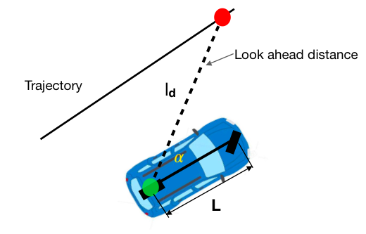
The target point is selected as the red point in the above figure. And the distance between the rear axle and the target point is denoted as ld. Our target is to make the vehicle steer at a correct angle and then proceed to that point. So the geometric relationship figure is as follows, the angle between the vehicle's body heading and the look-ahead line is referred to as α. Because the vehicle is a rigid body and proceeds around the circle. The instantaneous center of rotation(ICR) of this circle is shown as follows and the radius is denoted as R.

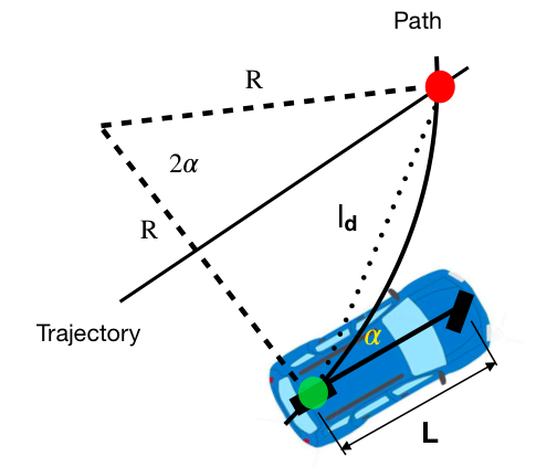
2.1 Pure Pursuit Formulation

From the law of sines:

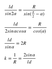
k is the curvature. Using the bicycle model (If you have no idea about the kinematic bicycle model, you can refer to another article named "Simple Understanding of Kinematic Bicycle Model"),

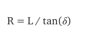
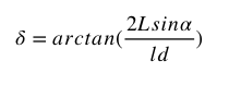
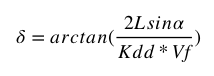
So the steering angle δ can be calculated as:

The pure pursuit controller is a simple control. It ignores dynamic forces on the vehicles and assumes the no-slip condition holds at the wheels. Moreover, if it is tuned for low speed, the controller would be dangerously aggressive at high speeds. One improvement is to vary the look-ahead distance ld based on the speed of the vehicle.

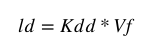
So the steering angle changed as:

2.2 Code sample for Pure Persuit Control

Here is the main code implementation of pure persuit control in Python. Waypoints[-1] refer to the target point. Yaw is the orientation of vehicle. We also need to add the max steering angle bounds.

# Pure Persuit Control
y_delta=waypoints[-1][1]-y
x_delta=waypoints[-1][0]-x
alpha=np.arctan(y_delta/x_delta)-yaw
                        
if alpha > np.pi/2:
    alpha -= np.pi
if alpha < - np.pi/2:
    alpha += np.pi 

steer_output=np.arctan(2*3*np.sin(alpha)/(self._kpp*v))
# Obey the max steering angle bounds
if steer_output>1.22:
    steer_output=1.22
if steer_output<-1.22:
    steer_output=-1.22

2.3 Pure Pursuit Simulation in CARLA

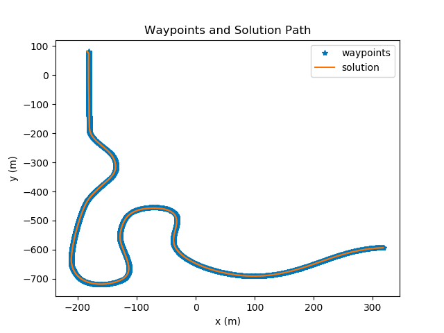
Now we know how to control the steering wheel. Let's see how the pure pursuit controller behaves in the CARLA simulator.

As you can see in the above result, we have successfully followed the race track and completed 100.00% of waypoints.

2.4 Why Pure Pursuit Controller is effective?

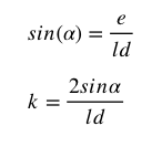
Let's see what is the cross-track error in this case. First, the cross-track error is defined as the lateral distance between the heading vector and the target point as follows. If the cross-track error is smaller, that means our vehicle follows the path better.

What is the relationship between the cross-track error and the curvature k? Before we have already known,

we can easily arrive,

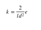
The above equation shows that the curvature k is proportional to the cross-track error. As the error increases, so does the curvature, bringing the vehicle back to the path more aggressively. The proportional gain 2/ld² can be tuned by yourself. In short, pure pursuit control works as a proportional controller of the steering angle operating on the cross-track error. The cross-track error can be reduced by controlling the steering angle, so this method works.

3. Stanley Controller

Secondly, we will discuss Stanley Controller. It is the path tracking approach used by Standford University's Darpa Grand Challenge team. Different from the pure pursuit method using the rear axle as its reference point, Stanley method use the front axle as its reference point. Meanwhile, it looks at both the heading error and cross-track error. In this method, the cross-track error is defined as the distance between the closest point on the path with the front axle of the vehicle.

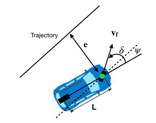
3.1 Stanley formulation

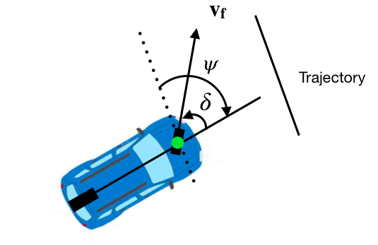
As you can see in figure above, ψ is heading error which refers to the angle between the trajectory heading and the vehicle heading. The steering angle is denoted as δ. There are three intuitive steering laws of Stanley method,

Firstly, eliminating the heading error. δ (t)= ψ(t)

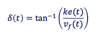
Secondly, eliminating the cross-track error. This step is to find the closest point between the path and the vehicle which is denoted as e(t). The steering angle can be corrected as follows,

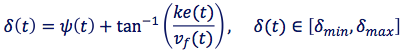
The last step is to obey the max steering angle bounds. That means δ(t)∈ [δ_min,δ_max]. So we can arrive,

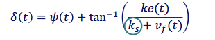
One adjustment of this controller is to add a softening constant to the controller. It can ensure the denominator be non-zero.

3.2 Code sample of Stanley Control

Below is the part of code implementation of Stanley control. I choose k=1.0. You can also test other values (e.g. 0.8, 0.7, 0.5, etc.).

#Code sample of Stanley Control
trajectory_yaw = self.get_global_yaw(waypoints[-1], waypoints[0])

# heading error
heading_error = trajectory_yaw - yaw
heading_error = self.get_valid_angle(heading_error)
            
# crosstrack error
e_r = 0
min_idx = 0
# Get the minmum distance between the vehicle and target trajectory
for idx in range(len(waypoints)):
    dis = self.get_dist(x,y,waypoints[idx][:2])
    if idx == 0:
       e_r = dis
    if dis < e_r:
        e_r = dis
        min_idx = idx

min_path_yaw = self.get_global_yaw(waypoints[min_idx],[x,y])
cross_yaw_error = min_path_yaw - yaw
cross_yaw_error = self.get_valid_angle(cross_yaw_error)
if cross_yaw_error > 0:
   e_r = e_r
else:
   e_r = -e_r
delta_error = np.arctan(1.0*e_r/(v+1.0e-6))
steer_output = heading_error + delta_error

3.3 Stanley Simulation in CARLA

After knowing how to control the steering angle, we now can make the vehicle follow a path. Let's first see how the Stanley method behaves in the CARLA simulator. As same as the pure pursuit before, we implement the above formulation to python and connect it with the CARLA simulator.

Using the Stanley controller, we can also complete 100.00% of waypoints. Moreover, looking at the video, the vehicle proceeds much more steadily than the Pure Pursuit controller, especially when it comes to a turn. We will discuss why the Stanley controller is effective and steady.

3.4 Why Stanley Controller is effective and steady?

Let's recap its formulation,

Stanley controller not only considers the heading error but also corrects the cross-track error. Let's look at these two scenarios,

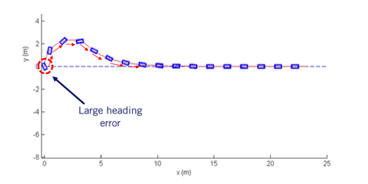
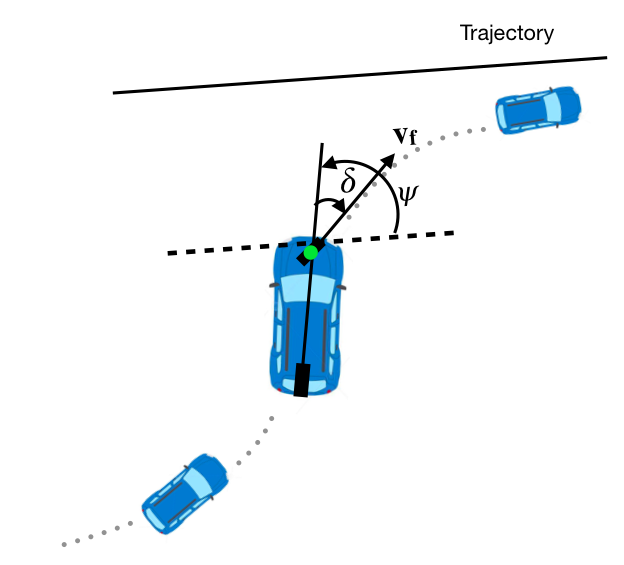
Firstly, if the heading error is large and cross-track error is small, that means ψ is large, so the steering angle δ will be large as well and steer in the opposite direction to correct the heading error, which can bring the vehicle orientation as same as the trajectory.

The process of this scenario can be drawn as below,

Secondly, if the cross-track error is large with small heading error, that can makes,

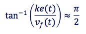
so the steering angle will be,

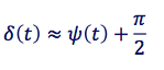
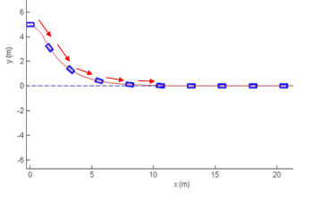
Supposing the heading error ψ(t) =0, δ(t) will be π/2. That makes the vehicle run towards the path as follows,

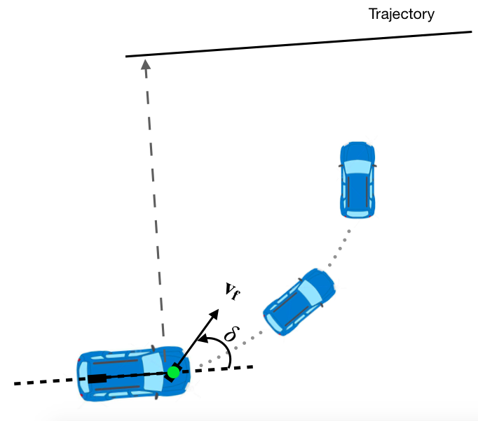
As the heading changes due to the steering angle, the heading correction counteracts the cross-track correction and drives the steering angle back to zero. When the vehicle approaches the path, cross-track error drops and the steering angle starts to correct the heading alignment as follows,

The process of this scenario can be drawn as follows,

In short, the Stanley controller is a simple but effective and steady method for later control. These two methods are both geometric controller. We will discuss another non-geometric controller which is the Model Predictive Controller known as MPC.

4. Model Predictive Controller

4.1 Cost Function

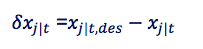
We should first know the cost function. For example, in this project, we want to control the vehicle to follow a race track. So the cost function should contain the deviation from the reference path, smaller deviation better results. Meanwhile, minimization of control command magnitude in order to make passengers in the car feel comfortable while traveling, smaller steering better results. This is similar to the optimization problem of optimal control theory and trades off control performance and input aggressiveness. Above these two targets, we can arrive the cost function as,

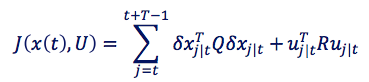
In the above equation, given the input of the steering angle, δx is the distance between the predictive point and the reference point as follows,

u is the steering input. So how can we know δx? We must have the predictive model of the plant first.

4.2 Predictive Model

The main concept of MPC is to use a model of the plant to predict the future evolution of the system[2]. In this case, we can use the simple kinematic bicycle model as follows, if you are not familiar with it, you can refer to my another blog.

x_dot = v * cos(δ + θ)

y_dot = v * sin(δ + θ)

θ_dot = v / R = v / (L/sin(δ)) = v * sin(δ)/L

δ_dot = φ

x_(t+1) = x_t + x_dot * Δt

y_(t+1) = y_t + y_dot * Δt

θ_(t+1) = θ_t + θ_dot * Δt

δ_(t+1) = δ_t + δ_dot * Δt

The states X are [x, y, θ, δ], θ is heading angle, δ is steering angle. Our inputs U are [ν, φ], ν is velocity, φ is steering rate.

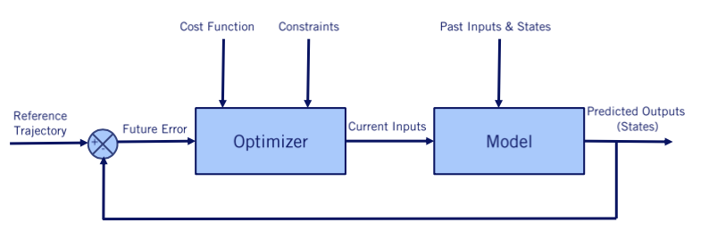
4.3 MPC Structure

Now, we have the cost function and the predictive model. The next step is to seek the best inputs to optimize our cost function. We can summarize the whole MPC process as follows,

So how to find the best control policy U? In this case, U is the steering angle.

1. Firstly, suppose our steering angle bounds are δ(t)∈ [δ_min, δ_max]. I use a simple method that discrete the input of the model, which is the steering angle δ into values with the same interval.
2. Then we can get the predicted outputs which are [x, y, θ, δ] using the above model and the input δ.
3. The last step is to select the smallest value of the cost function and its corresponding inputs δ. (In this case, we divided steering angle with 0.1 intervals from δ_min -1.2 to δ_max 1.2 radians. Then put it into the cost function and for loop to find the minimum value and its corresponding input δ.)
4. Repeat the above process in each time step.

4.4 Code sample of MPC

Here I use a simple way to get the minimum cost function J which is to discrete steering angle and calculate the min J and get corresponding steering angle.

# MPC control
# Discrete steering angle from -1.2 to 1.2 with interval of 0.1.
steer_list=np.arange(-1.2,1.2,0.1)
j_min = 0
for idx in range(len(steer_list)):
    vehicle_heading_yaw = yaw + steer_list[idx]
    t_diff = t - self.vars.t_previous
    pred_x = x + v*t_diff*np.cos(vehicle_heading_yaw)
    pred_y = y + v*t_diff*np.sin(vehicle_heading_yaw)
    delta_dis = self.get_dist(pred_x, pred_y, waypoints[-1][:2])
    j = 0.1*delta_dis**2 + steer_list[idx]**2
    if idx == 0:
       j_min = j
    if j < j_min:
       j_min = j
       steer_output = steer_list[idx]
# Obey the max steering angle bounds
if steer_output > 1.22:
   steer_output = 1.22
if steer_output < -1.22:
   steer_output = -1.22

4.5 MPC Implementation in CARLA simulator

Now we have our steering angle and know how to control the vehicle. Let's see how the MPC behaves in the CARLA simulator.

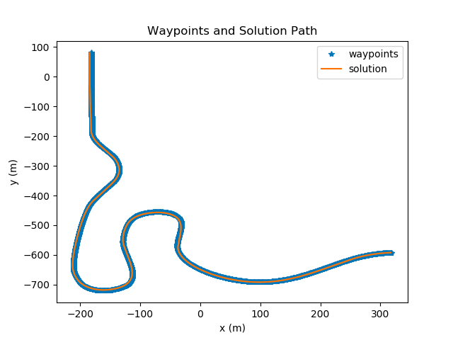
As you can see in the above figure, we can also complete 100% of waypoints with the MPC controller. But looking at the video, the vehicle runs not so steadily as using the Stanley Controller. Recap our cost function, we set the input δ in it because we do not want too big actions which may lead passengers feeling not good. I guess it is not appropriate just set like that. I think one method that can improve it is to make the action more continuous. If you are interested in it, you can try yourself. In this article, we just focus on the basic idea of MPC.

MPC has a lot of advantages. It can also be applied to linear or nonlinear models. It has a straightforward formulation and it can handle multiple constraints. For example, it can incorporate the low-level controller, adding constraints for Engine map, Fully dynamic vehicle model, Actuator models, Tire force models. And the cost function can be designed for different targets. For example, it can penalize collision, distance from the pre-computed offline trajectory, and the lateral offset from the current trajectory and so on. MPC is much more flexible and general. But it also has disadvantages of computationally expensive. Especially for the non-linear model, which is very general and even our bicycle model is also in this category, MPC must be solved numerically and cannot provide a closed-form solution.

5. Summary

In this article, we discussed three methods of lateral control and analyzed the project of trajectory tracking using these three methods. I hope it can give you some basic ideas for vehicle lateral control.

As respective to longitudinal control , I use PID control. I imported simple_pid in Python.

References

[1] Steven Waslander, Jonathan Kelly, "Introduction to Self-Driving Cars", Coursera.

[2] Gabriel M. Hoffmann, Claire J. Tomlin, "Autonomous Automobile Trajectory Tracking for Off-Road Driving: Controller Design, Experimental Validation and Racing", 2007.

[3] P. Falcone, F. Borrelli, J. Asgari, H. E. Tseng, D. Hrovat, "Predictive Active Steering Control for Autonomous Vehicle Systems", 2007.